Kinematic Equations: Complete Physics Guide

Executive Summary

Kinematic equations are four fundamental physics formulas that describe the motion of objects moving with constant acceleration, relating five key variables: initial velocity (v₀), final velocity (v), acceleration (a), time (t), and displacement (d). The key concept: these equations allow you to predict any aspect of an object's motion when you know at least three of the five variables, making them essential for calculating spacecraft trajectories, vehicle braking distances, and projectile paths. The four equations are: v = v₀ + at (velocity-time), d = v₀t + ½at² (position-time), v² = v₀² + 2ad (velocity without time), and d = ½(v₀ + v)t (average velocity).

Understanding which equation to use depends on identifying known and unknown variables in each problem. For example, calculating a rocket's velocity after launch requires knowing initial velocity, acceleration, and time - pointing to the first equation. Engineers use kinematic equations to design spacecraft trajectories, optimize vehicle safety systems, analyze sports performance, and program robotic motion controllers.

This guide provides step-by-step methods for solving kinematic problems, worked examples from free fall to projectile motion, and real-world applications in aerospace engineering and physics research.

Table of Contents

1. What are Kinematic Equations?

2. The Four Kinematic Equations

3. Understanding the Variables

4. How to Choose the Right Equation

5. Solving Kinematic Problems

6. Applications in Physics and Engineering

7. Common Mistakes to Avoid

8. FAQ

1. What are Kinematic Equations?

Kinematic equations describe the mathematical relationships between position, velocity, acceleration, and time for objects moving with constant acceleration. The term "kinematics" comes from the Greek word "kinema" meaning motion. These equations form the foundation of classical mechanics and apply to any object where acceleration remains constant throughout the motion period analyzed.

Constant Acceleration Assumption

The critical assumption underlying kinematic equations is constant acceleration. When acceleration varies with time or position, these simple equations no longer apply, requiring calculus-based approaches or numerical integration methods. Fortunately, many real-world scenarios involve constant or approximately constant acceleration:

• Free fall near Earth's surface: Gravitational acceleration remains constant at 9.8 m/s² (neglecting air resistance)

• Vehicle braking: Modern anti-lock braking systems maintain relatively constant deceleration

• Rocket launches: During initial ascent with consistent thrust and minimal air resistance

• Elevator motion: Controlled acceleration and deceleration phases

When acceleration changes significantly, the motion must be broken into segments where acceleration is approximately constant within each segment, similar to how chemists break complex reactions into individual stoichiometric steps to analyze them systematically.

Five Key Variables

Every kinematic problem involves five variables, and kinematic equations relate different combinations of these variables:

1. v₀ - Initial velocity (starting speed and direction)

2. v - Final velocity (ending speed and direction)

3. a - Acceleration (rate of velocity change)

4. t - Time (duration of motion)

5. d - Displacement (position change)

Each of the four kinematic equations uses exactly four of these five variables, omitting one. This structure allows you to solve for any unknown variable when you know three others, providing flexibility in problem-solving approaches.

2. The Four Kinematic Equations

Equation 1: Velocity with Time

v = v₀ + at

This equation relates final velocity, initial velocity, acceleration, and time. It omits displacement (d).

Use when: You know or want to find velocity, and time is a known or desired variable.

Example: A spacecraft accelerates from rest at 5 m/s² for 10 seconds. What is its final velocity?

• v₀ = 0 m/s (from rest)

• a = 5 m/s²

• t = 10 s

• v = 0 + (5)(10) = 50 m/s

This straightforward equation derives directly from the definition of acceleration as the rate of velocity change: a = Δv/Δt, rearranged to Δv = at.

Equation 2: Position with Time

d = v₀t + ½at²

This equation relates displacement, initial velocity, time, and acceleration. It omits final velocity (v).

Use when: You need to find how far an object travels or where it ends up, and you know the time interval.

Example: A ball is thrown downward from a building at 5 m/s. How far does it fall in 3 seconds? (Use g = 10 m/s² for simplicity)

• v₀ = 5 m/s (downward, positive direction)

• a = 10 m/s² (gravity, downward)

• t = 3 s

• d = (5)(3) + ½(10)(3)² = 15 + 45 = 60 meters

The ½at² term represents the additional distance covered due to increasing velocity during acceleration, similar to how specific heat capacity calculations account for energy distribution during temperature changes.

Equation 3: Velocity without Time

v² = v₀² + 2ad

This equation relates final velocity, initial velocity, acceleration, and displacement. It omits time (t).

Use when: Time is unknown or not needed, but you know or want to find velocities and displacement.

Example: A car traveling at 20 m/s brakes with deceleration of 4 m/s² over 50 meters. What is its final velocity?

• v₀ = 20 m/s

• a = -4 m/s² (negative for deceleration)

• d = 50 m

• v² = (20)² + 2(-4)(50) = 400 - 400 = 0

• v = 0 m/s (the car stops)

This equation is particularly valuable in safety engineering where stopping distances matter more than stopping times.

Equation 4: Position without Initial Velocity

d = ½(v₀ + v)t

This equation relates displacement, initial velocity, final velocity, and time. It omits acceleration (a).

Use when: You know both velocities and time, or when working with average velocity.

This equation can be rewritten as d = v̄t where v̄ = ½(v₀ + v) is the average velocity. For constant acceleration, average velocity equals the arithmetic mean of initial and final velocities.

Example: An object accelerates from 10 m/s to 30 m/s over 4 seconds. How far does it travel?

• v₀ = 10 m/s

• v = 30 m/s

• t = 4 s

• d = ½(10 + 30)(4) = ½(40)(4) = 80 meters

5. Solving Kinematic Problems

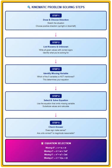
Step-by-Step Method

Step 1: Draw a diagram Sketch the situation. Mark initial position, final position, direction of motion, and direction of acceleration.

Step 2: Choose coordinate system Decide which direction is positive. Common choices: right/up = positive, left/down = negative. Be consistent throughout the problem.

Step 3: List knowns and unknowns Write down all given values with appropriate signs. Identify what you're solving for.

Step 4: Select appropriate equation Based on what's known and unknown, choose the equation that doesn't use the missing variable.

Step 5: Solve algebraically Rearrange equation if needed, substitute values, and calculate.

Step 6: Check answer Does the sign make sense? Are units correct? Is the magnitude reasonable?

Worked Example: Free Fall

Problem: A rock is dropped from a cliff 80 meters high. How long does it take to hit the ground? What is its velocity at impact? (Use g = 10 m/s²)

Solution - Part 1 (time):

Step 1: Diagram shows rock starting at cliff top, falling downward 80 m

Step 2: Choose downward as positive direction

Step 3: Knowns: v₀ = 0 (dropped), d = 80 m, a = 10 m/s²; Unknown: t; Missing: v

Step 4: Choose d = v₀t + ½at²

Step 5: Solve

• 80 = 0(t) + ½(10)t²

• 80 = 5t²

• t² = 16

• t = 4 seconds

Solution - Part 2 (impact velocity):

Step 3: Now know: v₀ = 0, a = 10 m/s², t = 4 s; Unknown: v

Step 4: Choose v = v₀ + at

Step 5: Solve

• v = 0 + (10)(4)

• v = 40 m/s

Check: Impact velocity 40 m/s (about 90 mph) seems reasonable for an 80-meter fall. Time of 4 seconds also reasonable.

Worked Example: Projectile Motion

Problem: A baseball is thrown upward at 25 m/s. How high does it go? (Use g = 10 m/s²)

Solution:

Step 1: Ball travels upward, slowing due to gravity, stops at maximum height

Step 2: Choose upward as positive; gravity acts downward (negative)

Step 3: Knowns: v₀ = 25 m/s (upward), v = 0 (at peak), a = -10 m/s² (gravity opposes motion); Unknown: d; Missing: t

Step 4: Choose v² = v₀² + 2ad

Step 5: Solve

• 0² = 25² + 2(-10)d

• 0 = 625 - 20d

• 20d = 625

• d = 31.25 meters

Check: About 31 meters (roughly 100 feet) seems reasonable for a ball thrown at 25 m/s (about 56 mph).

Worked Example: Vehicle Acceleration

Problem: A car accelerates from rest to 30 m/s over a distance of 150 meters. What is its acceleration? How long does this take?

Solution - Part 1 (acceleration):

Step 3: Knowns: v₀ = 0, v = 30 m/s, d = 150 m; Unknown: a; Missing: t

Step 4: Choose v² = v₀² + 2ad

Step 5: Solve

• 30² = 0² + 2a(150)

• 900 = 300a

• a = 3 m/s²

Solution - Part 2 (time):

Step 3: Now know: v₀ = 0, v = 30 m/s, a = 3 m/s²; Unknown: t

Step 4: Choose v = v₀ + at

Step 5: Solve

• 30 = 0 + 3t

• t = 10 seconds

Check: Acceleration of 3 m/s² and time of 10 seconds are both reasonable for a car accelerating from rest to highway speed.

6. Applications in Physics and Engineering

Spacecraft Trajectory Calculations

Kinematic equations form the foundation for calculating spacecraft trajectories during launch and landing phases where thrust provides approximately constant acceleration.

Launch phase analysis: During initial ascent, rockets experience relatively constant acceleration as engines burn fuel at steady rates. Engineers use kinematic equations to predict velocity and altitude at specific times, ensuring the spacecraft reaches required orbit insertion conditions.

Example: A rocket accelerates at 20 m/s² for 150 seconds during launch. Using v = v₀ + at with v₀ = 0:

• Final velocity: v = 0 + (20)(150) = 3,000 m/s (about 6,700 mph)

• Altitude reached: d = ½at² = ½(20)(150)² = 225,000 meters (225 km)

Landing calculations: Mars rovers use kinematic equations during descent phase when retrorockets provide constant deceleration. Mission planners calculate required deceleration rates and fuel consumption to ensure safe landing velocities.

The precision required in these calculations parallels the accuracy needed in stoichiometric calculations for spacecraft propellant chemistry.

Vehicle Safety Testing

Automotive engineers apply kinematic equations extensively in safety system design and crash testing.

Braking distance analysis: Determining minimum stopping distances requires solving for displacement given initial velocity and deceleration:

d = v²/(2a) (rearranged from v² = v₀² + 2ad with v = 0)

Example: Highway speed of 30 m/s (about 67 mph) with maximum braking deceleration of 7 m/s²:

• Stopping distance: d = (30)²/(2×7) = 900/14 ≈ 64 meters

This informs following distance guidelines and emergency brake system designs.

Airbag deployment timing: Crash sensors detect sudden deceleration. Kinematic equations calculate time until impact, triggering airbag inflation at the precise moment for maximum protection.

Sports Physics

Athletes and coaches use kinematic principles to optimize performance.

Vertical jump analysis: Using v² = v₀² + 2ad, the takeoff velocity needed for a target jump height is:

v₀ = √(2gh)

For a 1-meter jump with g = 10 m/s²: v₀ = √(2×10×1) = √20 ≈ 4.5 m/s takeoff velocity.

Projectile optimization: In sports like shot put, javelin, and basketball, launch angle and velocity determine range. While simplified kinematic equations assume no air resistance, they provide baseline predictions refined with experimental data.

Robotics and Automation

Industrial robots require precise motion control, using kinematic equations to plan trajectories that minimize time while respecting acceleration limits.

Motion planning: A robotic arm moving between positions must accelerate from rest, travel at constant velocity, then decelerate to rest. Kinematic equations calculate required distances for each phase:

• Acceleration phase: d₁ = ½at²

• Constant velocity phase: d₂ = vt

• Deceleration phase: d₃ = v²/(2a)

Total distance must match the specified movement, with time minimized for productivity.

Much like how understanding ionic versus covalent bonding determines material properties, choosing appropriate motion profiles determines robot performance characteristics.

8. FAQ

What are the four kinematic equations?

The four kinematic equations are: (1) v = v₀ + at relating final velocity, initial velocity, acceleration, and time; (2) d = v₀t + ½at² relating displacement, initial velocity, time, and acceleration; (3) v² = v₀² + 2ad relating velocities, acceleration, and displacement without time; and (4) d = ½(v₀ + v)t relating displacement, both velocities, and time without acceleration. Each equation uses exactly four of the five kinematic variables (initial velocity, final velocity, acceleration, time, displacement), omitting one variable. This structure allows you to solve for any unknown variable when you know three others. These equations apply only when acceleration is constant throughout the motion period analyzed. They are fundamental tools in physics for analyzing motion of objects from falling bodies to spacecraft trajectories.

How do you know which kinematic equation to use?

Choose the kinematic equation based on which variable is missing from your problem - either unknown and not needed, or not provided. First, list what you know and what you need to find. Count three known variables plus one unknown. Then identify which of the five variables (v₀, v, a, t, d) is neither given nor asked for - this missing variable determines your equation. Use v = v₀ + at when displacement is missing, d = v₀t + ½at² when final velocity is missing, v² = v₀² + 2ad when time is missing, and d = ½(v₀ + v)t when acceleration is missing. For example, if a problem gives initial velocity, time, and acceleration, and asks for displacement, the missing variable is final velocity, so use d = v₀t + ½at². This systematic approach ensures you select an equation containing only known quantities plus the single variable you are solving for.

What does constant acceleration mean in kinematic equations?

Constant acceleration means the rate of velocity change remains the same throughout the entire motion period being analyzed. The acceleration value does not change with time or position. This is the critical assumption underlying kinematic equations - if acceleration varies, these simple equations do not apply without modification. Real-world examples of approximately constant acceleration include: objects in free fall near Earth's surface where gravitational acceleration is constant at 9.8 m/s²; vehicles braking with anti-lock systems maintaining steady deceleration; rockets during initial launch with consistent thrust; and elevators during controlled acceleration phases. When acceleration changes significantly during motion, you must either break the motion into segments where acceleration is approximately constant within each segment, or use calculus-based methods. Many introductory physics problems specify constant acceleration explicitly or involve scenarios where this assumption is reasonable.

Can kinematic equations be used for circular motion?

Standard kinematic equations apply only to linear motion (motion along a straight line) with constant acceleration. They do NOT directly apply to circular motion because direction continuously changes in circular motion, making velocity and acceleration vectors change direction even if their magnitudes remain constant. Circular motion requires different equations involving angular velocity, angular acceleration, centripetal acceleration, and radius. However, you can use kinematic equations for the tangential component of motion if tangential acceleration is constant, treating it as one-dimensional motion along the circular path. For example, if a car speeds up while turning at constant radius, kinematic equations can describe how its speed changes along the curved path, but cannot describe the centripetal acceleration toward the circle's center. For uniform circular motion (constant speed), the magnitude of velocity is constant but its direction changes, so standard kinematic equations do not apply to the velocity vector itself.

What is the difference between distance and displacement in kinematics?

Distance is a scalar quantity measuring the total length of the path traveled, always positive, while displacement is a vector quantity measuring the straight-line change in position from start to finish, which can be positive, negative, or zero depending on chosen coordinate system and direction of motion. For example, if you walk 5 meters forward then 3 meters backward, the distance traveled is 8 meters (5 + 3), but displacement is only 2 meters forward (5 - 3). If you walk in a complete circle returning to your starting point, distance equals the circle's circumference, but displacement is zero because you ended where you began. Kinematic equations use displacement (d), not distance. This matters when objects reverse direction - a ball thrown upward then caught at release height has zero displacement despite traveling the sum of up and down distances. Always use displacement in kinematic calculations to get correct results.

How do you solve projectile motion problems with kinematic equations?

Solve projectile motion by separating it into independent horizontal and vertical components, applying kinematic equations to each direction separately. Horizontal motion has zero acceleration (neglecting air resistance), so velocity remains constant: d_x = v₀xt. Vertical motion has constant acceleration due to gravity: use all four kinematic equations with a = -g (if upward is positive). The key insight: horizontal and vertical motions share the same time t, which links the two directions. Typical approach: (1) Resolve initial velocity into horizontal (v₀x = v₀cosθ) and vertical (v₀y = v₀sinθ) components. (2) Analyze vertical motion to find time using d_y = v₀yt - ½gt². (3) Use this time in horizontal equation to find range. At maximum height, vertical velocity is zero. Landing occurs when vertical displacement returns to launch height. This decomposition method transforms complex two-dimensional motion into two simpler one-dimensional problems, each solvable with standard kinematic equations.

Related Articles

Continue exploring physics, engineering, and scientific calculations:

• Specific Heat Capacity: Complete Guide - Thermal physics and energy calculations

• Molar Mass: Complete Calculation Guide - Systematic calculation methods applicable to physics

• Stoichiometry: Complete Guide with Examples - Problem-solving strategies for quantitative science

• Polyatomic Ions: Complete List & Guide - Formula logic and systematic approaches

• Ionic vs Covalent Bonds: Complete Guide - Understanding fundamental science principles

Sources and References

1. Kinematics - Wikipedia. Fundamental equations and motion analysis. Wikipedia article

2. Equations of Motion - Wikipedia. Derivations and applications of kinematic equations. Wikipedia article

3. Classical Mechanics - Wikipedia. Theoretical foundations and principles. Wikipedia article

4. Chemistry: The Science in Context - Thomas R. Gilbert, Rein V. Kirss, Natalie Foster, Stacey Lowery Bretz. Physics and chemistry textbook covering motion and energy. Free PDF

5. The Role of Industrial Chemistry in Modern Manufacturing - Applications in engineering and materials science. Open Access PDF